![]()
In an electronic circuit, the impedance associated with that circuit is dependent on the circuit elements as well as the frequency of operation. For circuit elements with passive components, the impedance has always a real part equal to or greater than zero. The imaginary part can be inductive or capacitive. As the frequency is varied, the real and imaginary parts of the impedance may also vary and the reactive part may change from inductive to capacitive value.
If one now tries to place these impedances on a complex Z plane where the real axis is the Re(Z) and the Imagineary axis is Im(Z), they will fall within the right half plane of the complex plane. Considering the many possible impedance values, it will not be practical to use such a plane for impedance represenation.
To represent all possible impedances Z=R+jX on a complex plane is almost impossible.The impedance for Passive loads has a Real Part that takes on values from 0(zero) to +oo(infinity) and the Imaginary Part may vary from -oo to +oo.
For example if a transmission line is connected to a load and the length of the line is varied over a wide range, there will result many possible impedances.To deal with all these problems and with added benefits,
![]()
To make the Smith chart universal, that is irrespective of the characteristic imepadance used, normalized impedances are used. That is z=r+jx=(R+jX)/Zc.
For example, all impedances with Re(z)>=0.0 irrespective of the imaginary part (which may take values from -• to +• ) , lie on a circle with radius=1.0 as shown in the figure below. Other constant r and x values transform into circles with different radii and diferent center locations.
In the figure below the normalized resistances and reactances are shown with bars over R and X. They will be represented in the text by lower case letters {r and x}.

For impedances z = r + j x with positive real parts, that is for r >= 0.0 (all passive impedance elements), corresponding impedances lie inside the Smith chart (Yellow circular area). They all have a reflection coefficient magnitude rho between 0.0 and 1.0.
In this case, since maximum magnitude of |G|=rho is equal to 1.0, the radius of the Smith Chart is 1.0 whatever the geomterical size of the Smith chart is.
If an impedance z has a negative real part (negative resistance, or an active source), the corresponding impedance lies outside the Smith chart (Greenish areas). Note all impedances with negative real parts ( z = -r + j x , that is r < 0.0) have a reflection coefficient magnitude r = |G| > 1.0.
The reflection coefficent is related to the terminated impedance and is given by
![]()
Here GL is a complex number and written as u+jv.
![]()
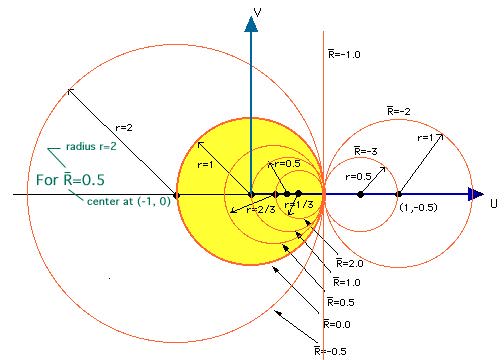
This is the equation of a circle with center at {u=r/(1+r) and v=0.0} and radius rad=1/(1+r)
For various r values, u, v and rad values are given in the following table.
| r | 0.00 | 0.50 | 1.00 | 2.00 | oo | -0.5 | -2.0 | -3.0 | -4.0 | u | 0.0 | 0.33 | 0.50 | 0.67 | 1.00 | -1.0 | 2.0 | 1.50 | 1.33 |
| v | 0.00 | 0.00 | 0.00 | 0.00 | 0.00 | 0.00 | 0.00 | 0.00 | 0.00 |
| rad | 1.00 | 0.67 | 0.50 | 0.33 | 0.00 | 2.00 | 1.00 | 0.50 | 0.33 |
Smith Chart animation showing the transformation of real part of the impedance into circles in the Smith Chart
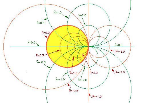
In the figure below, contant r circles are drawn for various r values. Note that for r=Real(Z/Zc)>=0.0, all loci of constant resistances fall within the yellow circular area. For r=Real(Z/Zc)<0.0, they fall outside the yellow circular area.
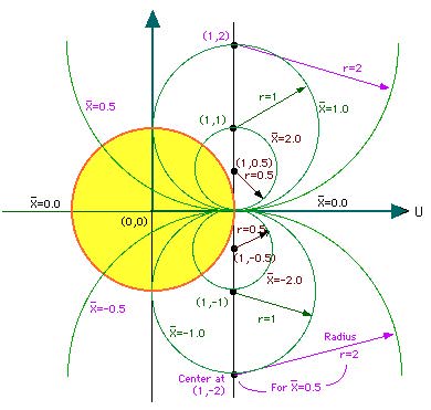
In a smilar manner, if the r values are eliminated and the resulting equation is written in terms of x values, the following equation is obtained.
This equation is also a circle with center at { u=1.0 and v=1/x } and radius rad=1/|x|.
For various x values, u, v and rad values are given in the following table
| x | 0.00 | 0.50 | 1.00 | 2.00 | 3.00 | oo | -2.0 | -1.0 | -0.5 | u | 1.00 | 1.00 | 1.00 | 1.00 | 1.00 | 1.00 | 1.00 | 1.00 | 1.00 |
| v | oo | 2.00 | 1.00 | 0.50 | 0.33 | 0.00 | -0.5 | -1.0 | -2.0 |
| rad | oo | 2.00 | 1.00 | 0.50 | 0.33 | 0.00 | 0.50 | 1.00 | 2.00 |
Smith Chart animation showing the transformation of Imaginary part of the Impedance into circles in the Smith Chart
In the figure below, contant x circles are drawn for various x values. Note that all loci of constant +x (inductive reactance) fall above u=0 and with -x (capacitive reactance), fall below the u=0.
 ;
;
Yellow circular region is usually referred to as the
and the rest is known as
A Highly Enlarged Smith Chart to see in detail the different parts of the Smith Chart.
)
)
)