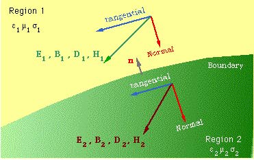
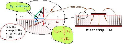
The changes in the field components from one medium to the other should be known. But these changes, that is the waves reflected and transmitted, should be consistent with Maxwell's equations.

Figure below shows two media seperated by a boundary.

Let

• n be the normal to the surface at the point of interest.
• E₁,D₁,H₁,B₁ be the fields in Medium I at the boundary
• E₂,D₂,H₂,B₂ be the fields in Medium II at the boundary
• Any of these vectors can be decomposed into two components at the boundary; a tangential component (parallel to the surface) and a normal component (perpendicular to the surface). For example, E₁ can be decomposed into E_1t and E_1n.

Tangential Component of E : Tangential Component of E field is Continuous

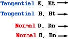
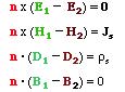
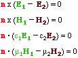
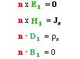
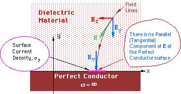
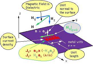
Tangential Component of H : Tangential Component of H field changes by the Infintitesimal Current density J_s if present at the boundary

Normal Component of D : Normal Component of D field changes by the surface current density s_s if present at the boundary

Normal Component of B : Normal Component of B field is continuous at the boundary

• General Case
• Dielectric - Dielectric interface (no surface charge and no surface current density)
• Dielectric - Perfect Conductor interface (fields inside the perfect conductor are zero)

Boundary Conditions
Field Components			General Conditions			Dielectric Boundary			Perfect Conductor

Examples:

• Microstrip Line (Dielectric Boundary)
  

  Note

  • Parallel (Tangential to the boundary) Component of the E field (E_|| or E_tan) is continuous (Same in the two regions) at the boundary.
  • Perpendicular Component of the E field has changed by (1/2) in magnitude (due to the continuity of D normal, i.e., D_n1=D_n2 or e₁E_^1=e₂E_^2)
  • The direction of the field has changed from q₁ to q₂.

  ---

• Perfect Conductor

  Electric Field:

  • Fields inside the perfect conductor are all zero.
  • As shown in the figure above, on the conductor surface, there is only a normal component of E field. In this case, only E_y is present at the conductor surface.
  • The surface charge density is given by s_s=n.D_n. In this case s_s=a_y.e(E_ya_y)=eE_y (Coul/m²).

  ---

  

  Magnetic Field

  • Assume that the H field in the dielectric is given as shown in the figure above. On the conductor surface, the normal B (therefore normal H) is zero. In this example: H_z=0|_z=0.
  • The surface current density is given by J_s=n x H|_{at conductor surface}. In this case J_s=a_z x (H_y+H_z)|_z=0 =H_ya_x (A/m).

Rectangular Waveguide

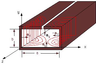
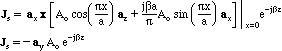
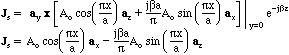
A rectangular Waveguide with inner dimensions (a,b) (y=0 to b and x=0 to a) is shown in the figure.The magnetic field for the TE₁₀ mode is given by

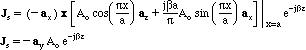
We can find the current density on the inner conductor walls from

The current density at x=0 as a function of y is calculated from

Note that the current density is constant on this wall.
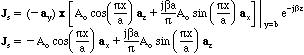
The current density at x=a for any y is calculated from

Note that the current density is also constant on this wall.
The current density at y=0 as a function of x is calculated from

The current density at y=b as a function of x is calculated from

The current density is plotted in the figure for half a wavelength along the z-direction and it repeats itself along the z-axis. Note that the curent density (therefore, the current) is zero at x=a/2 both at the upper and lower walls. A slot opened at this position along the z-axis will not alter the field pattern as well as the current flow on the waveguide. A slot on the upper or lower walls may be used to insert a probe into the waveguide to monitor the strength of the propogating fields as well as the standing wave ratio on a line.